Inside StarRocks: Why Joins Are Faster Than You’d Expect

StarRocks takes the opposite approach: keep data normalized and make joins fast enough to run on the fly. The challenge is the plan. In a distributed system, the join search space is huge, and a good plan can be orders of magnitude faster.

This deep dive explains how StarRocks’ cost-based optimizer makes that possible, in four parts: join fundamentals and optimization challenges, logical join optimizations, join reordering, and distributed join planning. Finally, we examine real-world case studies from NAVER, Demandbase, and Shopee to illustrate how efficient join execution delivers tangible business value.

Join Fundamentals and Optimization Challenges

1.1 Join Types

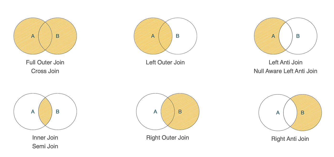
The diagram above illustrates several common join types:

• Cross Join: Produces a Cartesian product between the left and right tables.
• Full / Left / Right Outer Join: For rows that do not find a match, outer joins return results with NULL values filled in according to the join semantics—on both tables (full), the left table (left), or the right table (right).
• Anti Join: Returns rows that do not have a matching counterpart in the join relationship. Anti-joins typically appear in query plans for NOT IN or NOT EXISTS subqueries.
• Semi Join: The opposite of an anti-join, it returns only rows that do have a match in the join relationship, without producing duplicate result rows from the matching side.
• Inner Join: Returns the intersection of the left and right tables. Based on the join condition, it may generate one-to-many result rows.

1.2 Challenges in Join Optimization

Join performance optimization generally falls into two areas:

• improving the efficiency of join operators on a single node, and
• designing a reasonable join plan that minimizes input size and execution cost.

This article focuses on the second aspect. To set the stage, we begin by examining the key challenges in join optimization.

Challenge 1: Multiple Join Implementation Strategies

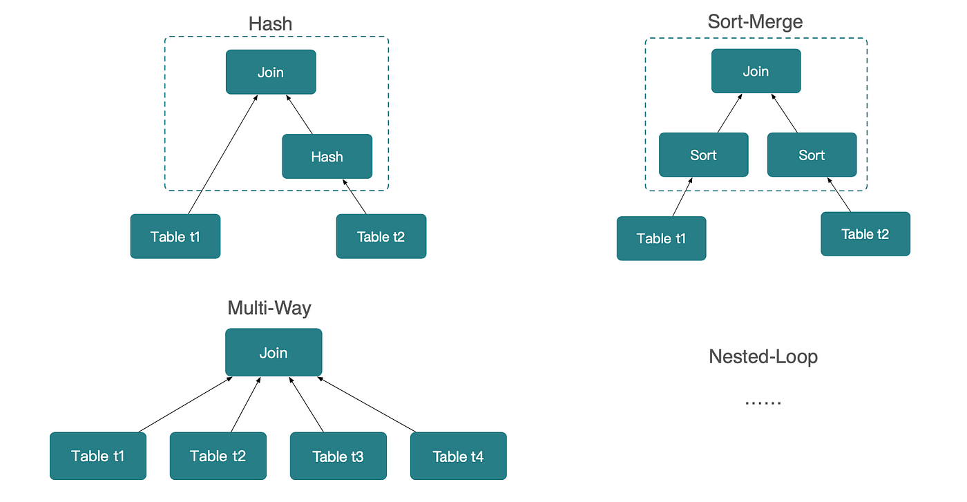
As shown above, different join algorithms perform very differently depending on the scenario. For example, Sort-Merge Join can be significantly more efficient than Hash Join when operating on already sorted data. However, in distributed databases where data is typically hash-partitioned, Hash Join often outperforms Sort-Merge Join by a wide margin. As a result, the database must choose the most appropriate join strategy based on the specific workload and data characteristics.

Challenge 2: Join Order Selection in Multi-Table Joins

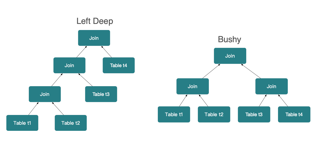
In multi-table join scenarios, executing highly selective joins first can significantly improve overall query performance. However, determining the optimal join order is far from trivial.

As illustrated above, under a left-deep join tree model, the number of possible join orders for N tables is on the order of 2^n-1. Under a bushy join tree model, the number of possible combinations grows even more dramatically, reaching 2^(n-1) * C(n-1). For a database optimizer, the time and cost required to search for the optimal join order therefore increases exponentially, making join ordering one of the most challenging problems in query optimization.

Challenge 3: Difficulty in Estimating Join Effectiveness

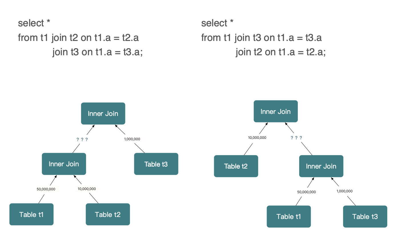
Before query execution, it is extremely difficult for the database to accurately predict the real execution behavior of a join. A common assumption is that joining a small table with a large table is more selective than joining two large tables, but this is not always true.

In practice, one-to-many relationships are common, and in more complex queries, joins are often combined with filters, aggregations, and other operators. After data flows through multiple transformations, the optimizer’s ability to accurately estimate join input sizes and selectivity degrades significantly.

Challenge 4: A Single-Node Optimal Plan Is Not Necessarily Optimal in Distributed Systems

Press enter or click to view image in full size

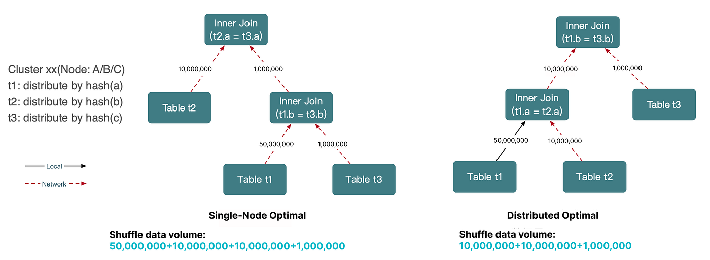
In distributed systems, data often needs to be reshuffled or broadcast across nodes so that the required records can participate in join computation. Distributed joins are no exception.

This introduces a key complication: an execution plan that is optimal in a single-node database may perform poorly in a distributed environment because it ignores data distribution and network transfer costs.

Therefore, when planning join execution strategies in distributed databases, the optimizer must explicitly account for data placement and communication overhead in addition to local execution efficiency.

1.3 SQL Optimization Workflow

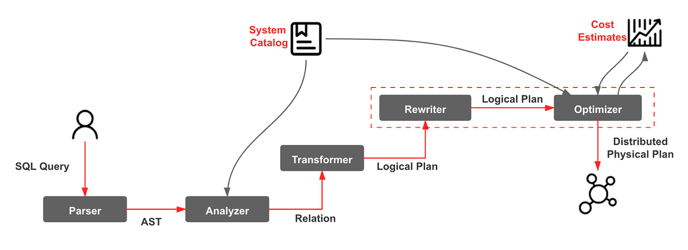
In StarRocks, SQL optimization is primarily handled by the query optimizer and is mainly concentrated in the Rewrite and Optimize phases.

1.4 Principles of Join Optimization

At present, StarRocks primarily uses Hash Join as its join algorithm. By default, the right-hand table is used to build the hash table. Based on this design choice, we summarize five key optimization principles:

1. Different join types have very different performance characteristics. Whenever possible, prefer higher-performance join types and avoid expensive ones. Based on the typical size of join outputs, the rough performance ranking is: Semi Join / Anti Join > Inner Join > Outer Join > Full Outer Join > Cross Join.
2. When using Hash Join, building the hash table on a smaller input is significantly more efficient than building it on a large table.
3. In multi-table joins, prioritize joins with high selectivity.
4. Minimize the amount of data participating in joins whenever possible.
5. Minimize network overhead introduced by distributed joins.

Join Logical Optimization

This section introduces a set of heuristic rules used by StarRocks to optimize joins at the logical level.

2.1 Type Transformations

The first group of optimizations directly follows the first join optimization principle discussed earlier: transform low-efficiency join types into more efficient ones whenever the semantics allow it.

StarRocks currently applies three major transformation rules.

Rule 1: Converting a Cross Join into an Inner Join

A Cross Join can be rewritten as an Inner Join when it satisfies the following condition:

• There exists at least one predicate that expresses a join relationship between the two tables.

For example:

-- Before transformation
SELECT * FROM t1, t2 WHERE t1.v1 = t2.v1

-- After transformation
-- WHERE t1.v1 = t2.v1 is a join predicate
SELECT * FROM t1 INNER JOIN t2 ON t1.v1 = t2.v1;

Rule 2: Converting an Outer Join into an Inner Join

A Left / Right Outer Join can be rewritten as an Inner Join when the following conditions are met:

• There exists a predicate referencing the nullable side of the outer join (Right table for a Left Outer Join, or Left table for a Right Outer Join).
• The predicate is a strict (null-rejecting) predicate.

Example:

-- Before transformation
SELECT * FROM t1 LEFT OUTER JOIN t2 ON t1.v1 = t2.v1 WHERE t2.v1 > 0;

-- After transformation
-- t2.v1 > 0 is a strict predicate on t2
SELECT * FROM t1 INNER JOIN t2 ON t1.v1 = t2.v1 WHERE t2.v1 > 0;

⚠️ Important note: In an outer join, ON clause predicates participate in null extension, not filtering. Therefore, this rule does not apply to join predicates inside the ON clause:

SELECT * FROM t1 LEFT OUTER JOIN t2 ON t1.v1 = t2.v1 AND t2.v1 > 1;

This query is not semantically equivalent to:

SELECT * FROM t1 INNER JOIN t2 ON t1.v1 = t2.v1 AND t2.v1 > 1;

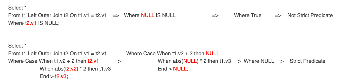
This introduces the concept of strict (null-rejecting) predicates. In StarRocks, a predicate that filters out NULL values is considered a strict predicate, for example a > 0. Predicates that do not eliminate NULL values are classified as non-strict predicates, such as a IS NULL. Most predicates fall into the strict category; non-strict predicates are primarily those involving IS NULL, IF, CASE WHEN, or certain function-based expressions.

To determine whether a predicate is strict, StarRocks uses a simple yet effective approach: all referenced columns are replaced with NULL, and the expression is then simplified. If the result evaluates to TRUE, it means the WHERE clause does not filter out rows with NULL inputs, and the predicate is therefore non-strict. Conversely, if the result evaluates to FALSE or NULL, the predicate is considered strict.

Rule 3: Converting a Full Outer Join into a Left / Right Outer Join

A Full Outer Join can be rewritten as a Left Outer Join or Right Outer Join when the following condition is satisfied:

• There exists a strict predicate that can be bound exclusively to the left or right table.

Example:

-- Before transformation
SELECT * FROM t1 FULL OUTER JOIN t2 ON t1.v1 = t2.v1 WHERE t1.v1 > 0;

-- After transformation
-- t1.v1 > 0 is a strict predicate on the left table
SELECT * FROM t1 LEFT OUTER JOIN t2 ON t1.v1 = t2.v1 WHERE t1.v1 > 0;

2.2 Predicate Pushdown

Predicate pushdown is one of the most important and commonly used join optimization techniques. Its primary purpose is to filter join inputs as early as possible, thereby reducing the amount of data involved in the join and improving overall performance.

For predicates in the WHERE clause, predicate pushdown can be applied—and may enable join type transformations—when the following conditions are satisfied:

• The join can be of any type.
• The WHERE predicate can be bound to one of the join inputs.

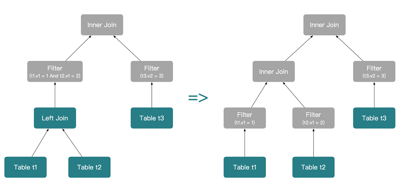
For example:

Select *  
From t1 Left Outer Join t2 On t1.v1 = t2.v1 
        Left Outer Join t3 On t2.v2 = t3.v2 
Where t1.v1 = 1 And t2.v1 = 2 And t3.v2 = 3;

The predicate pushdown process proceeds as follows.

Step 1 :

Push down (t1.v1 = 1 AND t2.v1 = 2) and (t3.v2 = 3) separately. Since the join type transformation rules are satisfied,(t1 LEFT OUTER JOIN t2) LEFT OUTER JOIN t3can be rewritten as (t1 LEFT OUTER JOIN t2) INNER JOIN t3.

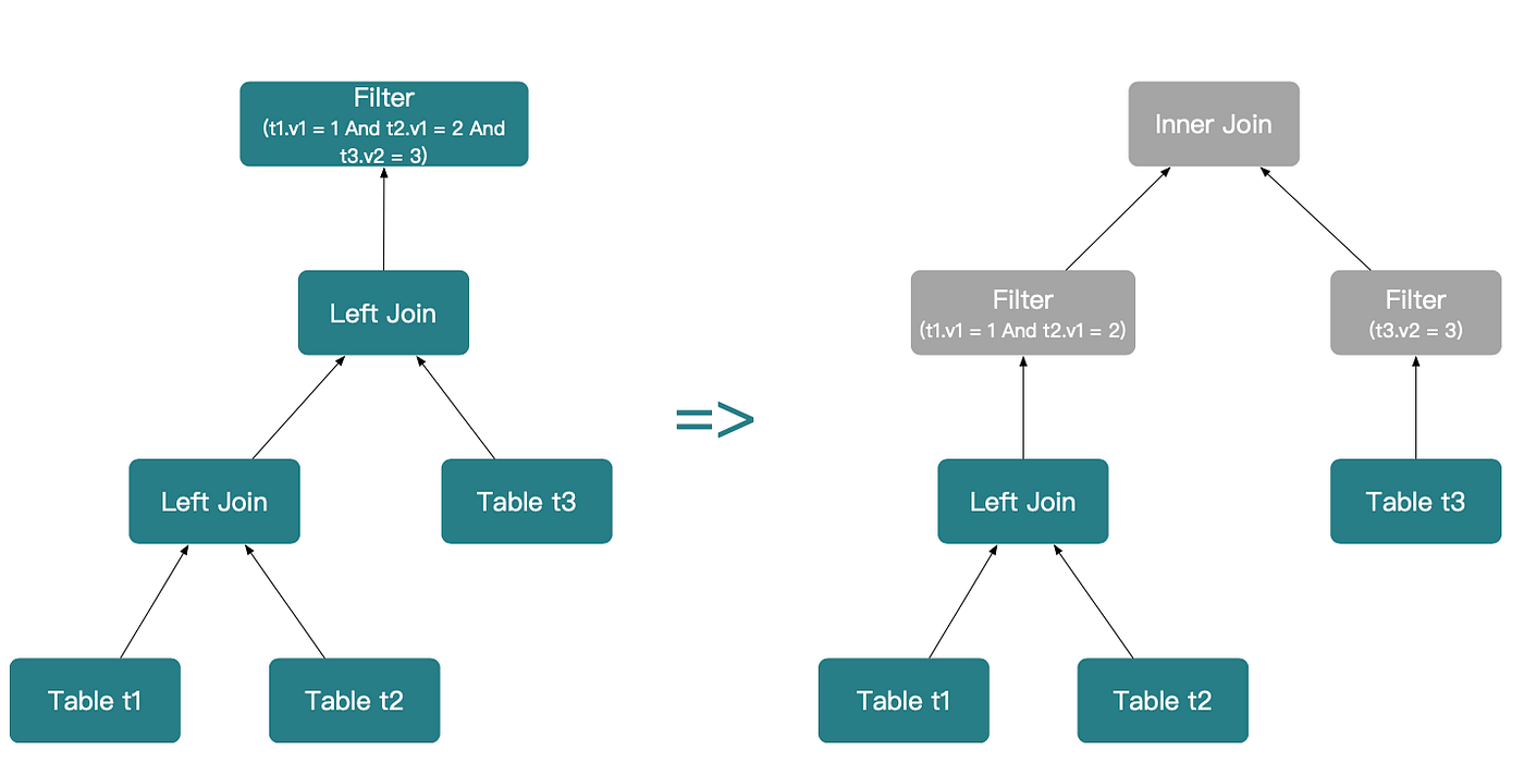
Step 2:

Continue pushing down (t1.v1 = 1) and (t2.v1 = 2). At this point,t1 LEFT OUTER JOIN t2 can be further transformed intot1 INNER JOIN t2.

It is important to note that predicate pushdown rules for join predicates in the ON clause differ from those for the WHERE clause. We distinguish between two cases: Inner Joins and other join types.

Case 1: Inner Join

For Inner Joins, pushing down join predicates in the ON clause follows the same rules as WHERE clause predicate pushdown. This has already been discussed above and will not be repeated here.

Case 2: Outer / Semi / Anti Joins

For Outer, Semi, and Anti Joins, predicate pushdown on ON clause join predicates must satisfy the following constraints, and no join type transformation is allowed during the pushdown process:

• The join must be a Left or Right Outer / Semi / Anti Join.
• The join predicate must be bindable only to the nullable side (the right input for a Left Join, or the left input for a Right Join).

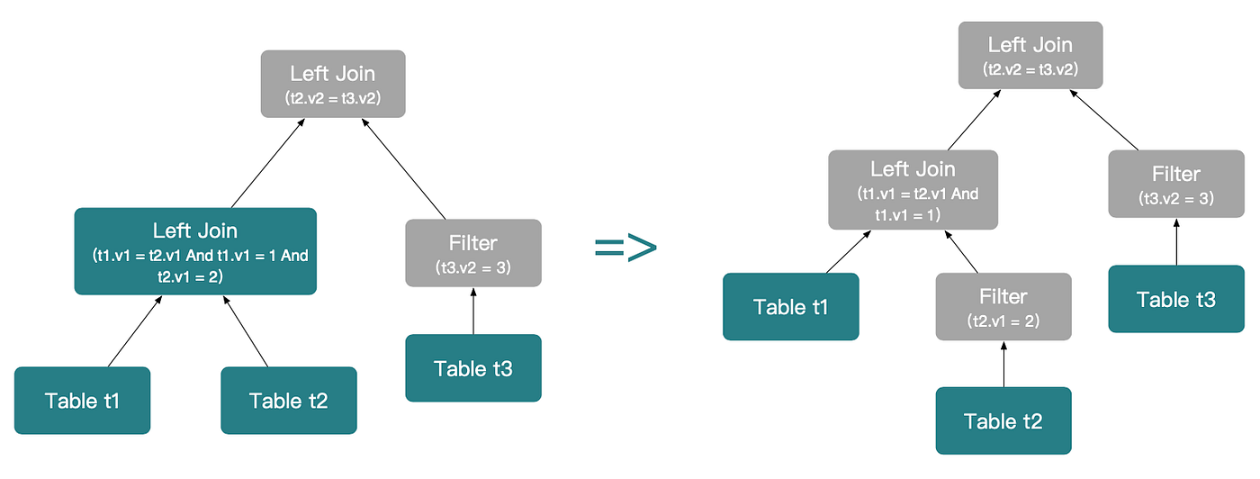
Consider the following example:

Select *  
From t1 Left Outer Join t2 On t1.v1 = t2.v1 And t1.v1 = 1 And t2.v1 = 2 
        Left Outer Join t3 On t2.v2 = t3.v2 And t3.v2 = 3;

The predicate pushdown proceeds as follows.

Step 1:

Push down the join predicate (t3.v2 = 3), which can be bound to the right input of t1 LEFT JOIN t2 LEFT JOIN t3. At this stage, the LEFT OUTER JOIN cannot be converted into an INNER JOIN.

Press enter or click to view image in full size

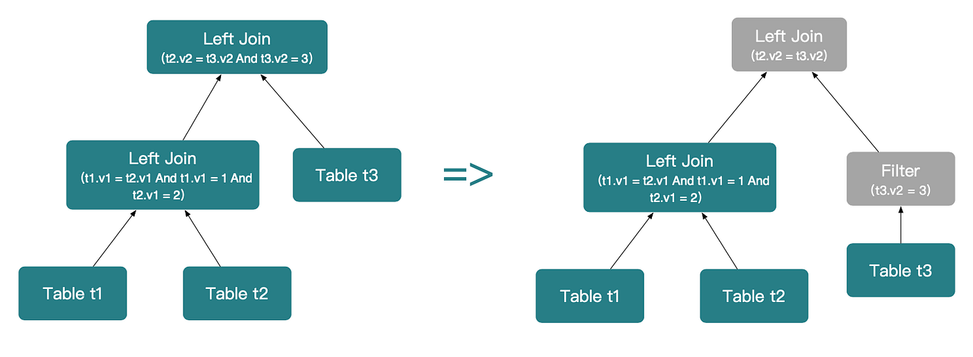
Step 2:

Push down the join predicate (t2.v1 = 2), which can be bound to the right input oft1 LEFT JOIN t2.

However, the predicate (t1.v1 = 1) is bound to the left input. Pushing it down would filter rows from t1, violating the semantics of a LEFT OUTER JOIN. Therefore, this predicate cannot be pushed down.

Press enter or click to view image in full size

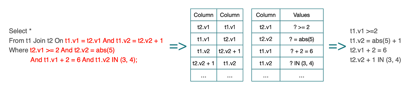
2.3 Predicate Extraction

In the predicate pushdown rules discussed earlier, only predicates with conjunctive semantics can be pushed down. For example, in t1.v1 = 1 AND t2.v1 = 2 AND t3.v2 = 3, each sub-predicate is connected by conjunction, making pushdown straightforward. However, predicates with disjunctive semantics, such ast1.v1 = 1 OR t2.v1 = 2 OR t3.v2 = 3, cannot be pushed down directly.

In real-world queries, disjunctive predicates are quite common. To address this, StarRocks introduces an optimization called predicate extraction (column value derivation). This technique derives conjunctive predicates from disjunctive ones by performing a series of union and intersection operations on column value ranges. The derived conjunctive predicates can then be pushed down to reduce join input size.

For example:

-- Before predicate extraction
SELECT *
FROM t1 JOIN t2 ON t1.v1 = t2.v1
WHERE (t2.v1 = 2 AND t1.v2 = 3)OR (t2.v1 > 5 AND t1.v2 = 4);

Using column value derivation on (t2.v1 = 2 AND t1.v2 = 3) OR (t2.v1 > 5 AND t1.v2 = 4), the optimizer can extract the following predicates:

• t2.v1 >= 2
• t1.v2 IN (3, 4)

The query can then be rewritten as:

SELECT *
FROM t1 JOIN t2 ON t1.v1 = t2.v1
WHERE (t2.v1 = 2 AND t1.v2 = 3)OR (t2.v1 > 5 AND t1.v2 = 4)AND t2.v1 >= 2
AND t1.v2 IN (3, 4);

It is important to note that the extracted predicates may form a superset of the original predicate ranges. As a result, they cannot safely replace the original predicates and must instead be applied in addition to them.

2.4 Equivalence Derivation

In addition to predicate extraction, another important predicate-level optimization is equivalence derivation. This technique leverages join equality conditions to infer value constraints on one side of the join from predicates applied to the other side.

Specifically, based on the join condition, value ranges on columns from the left table can be used to derive corresponding value ranges on columns from the right table, and vice versa.

For example:

-- Original SQL
SELECT *
FROM t1 JOIN t2 ON t1.v1 = t2.v1
WHERE (t2.v1 = 2 AND t1.v2 = 3)
   OR (t2.v1 > 5 AND t1.v2 = 4);

Using predicate extraction on (t2.v1 = 2 AND t1.v2 = 3) OR (t2.v1 > 5 AND t1.v2 = 4), the optimizer can derive the following predicates:

• t2.v1 >= 2
• t1.v2 IN (3, 4)

Resulting in:

SELECT *
FROM t1 JOIN t2 ON t1.v1 = t2.v1
WHERE (t2.v1 = 2 AND t1.v2 = 3)
   OR (t2.v1 > 5 AND t1.v2 = 4)
  AND t2.v1 >= 2
  AND t1.v2 IN (3, 4);

Next, using the join predicate (t1.v1 = t2.v1) together with t2.v1 >= 2, equivalence derivation can infer an additional predicate:

• t1.v1 >= 2

The query can therefore be further rewritten as:

SELECT *
FROM t1 JOIN t2 ON t1.v1 = t2.v1
WHERE (t2.v1 = 2 AND t1.v2 = 3)
   OR (t2.v1 > 5 AND t1.v2 = 4)
  AND t2.v1 >= 2
  AND t1.v2 IN (3, 4)
  AND t1.v1 >= 2;

Applicability and Constraints

The scope of equivalence derivation is more limited than predicate extraction. Predicate extraction can be applied to arbitrary predicates, whereas equivalence derivation, like predicate pushdown, has different constraints depending on the join type. As before, we distinguish between WHERE predicates and ON clause join predicates.

For WHERE predicates:

• There are almost no restrictions. Predicates can be derived from the left table to the right table and vice versa.

For ON clause join predicates:

• For Inner Joins, the rules are the same as for WHERE predicates—no additional constraints apply.
• For join types other than Inner Join, only Semi Joins and Outer Joins are supported, and derivation is one-directional only, opposite to the join direction:
• For a Left Outer Join, predicates can be derived from the left table to the right table.
• For a Right Outer Join, predicates can be derived from the right table to the left table.

Why Is Equivalence Derivation One-Directional for Outer / Semi Joins?

The reason is straightforward. Consider a Left Outer Join. As discussed in predicate pushdown rules, only predicates on the right table can be pushed down; predicates on the left table cannot, as doing so would violate the semantics of a left outer join.

For the same reason, predicates derived from the right table and applied to the left table must also respect this constraint. In practice, such derived predicates on the preserved side do not help filter data early and instead introduce additional evaluation overhead. Therefore, equivalence derivation for Outer and Semi Joins is intentionally restricted to a single direction.

Implementation Details

StarRocks implements equivalence derivation by maintaining two internal maps:

• One map tracks column-to-column equivalence relationships.
• The other map tracks column-to-value or column-to-expression equivalences.

By performing lookups and inference across these two maps, the optimizer derives additional equivalent predicates. The overall mechanism is illustrated below:

2.5 Limit Pushdown

In addition to predicates, LIMIT clauses can also be pushed down through joins. When a query involves an Outer Join or a Cross Join, the LIMIT can be pushed down to child operators whose output row count is guaranteed to be stable.

For example, in a Left Outer Join, the output row count is at least the same as that of the left input. Therefore, the LIMIT can be pushed down to the left table (and symmetrically for a Right Outer Join).

-- Before pushdown
SELECT *
FROM t1 LEFT OUTER JOIN t2 ON t1.v1 = t2.v1
LIMIT 100;

-- After pushdown
SELECT *
FROM (SELECT * FROM t1 LIMIT 100) t
LEFT OUTER JOIN t2 ON t.v1 = t2.v1
LIMIT 100;

Special Cases: Cross Join and Full Outer Join

A Cross Join produces a Cartesian product, with output cardinality equal torows(left) × rows(right). A Full Outer Join produces at leastrows(left) + rows(right).

For these join types, a LIMIT can be pushed down to both inputs independently:

-- Before pushdown
SELECT *
FROM t1 JOIN t2
LIMIT 100;

-- After pushdown
SELECT *
FROM (SELECT * FROM t1 LIMIT 100) x1
JOIN (SELECT * FROM t2 LIMIT 100) 
LIMIT 100;

Join Reordering

Join reordering is used to determine the execution order of multi-table joins. The optimizer aims to execute high-selectivity joins as early as possible, thereby reducing the size of intermediate results and improving overall query performance.

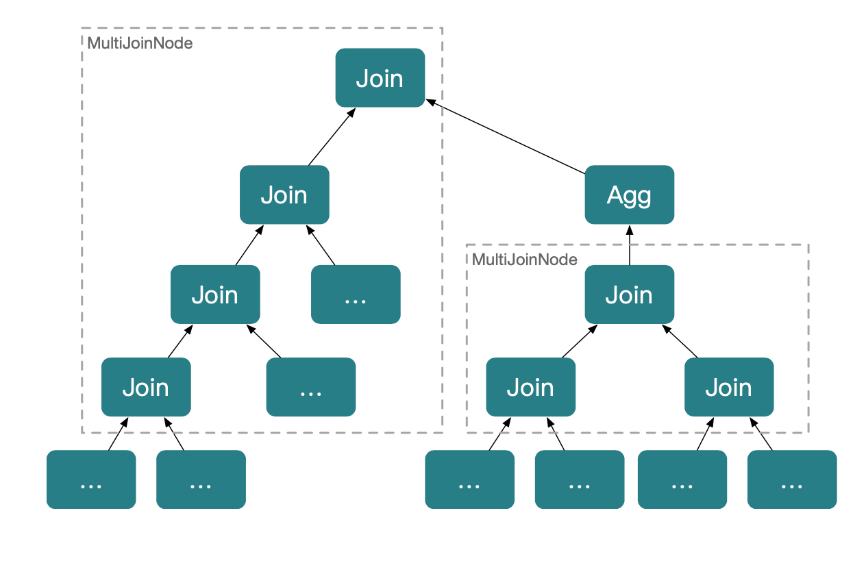
In StarRocks, join reordering primarily operates on continuous sequences of Inner Joins or Cross Joins. As illustrated below, StarRocks groups a sequence of consecutive Inner / Cross Joins into a Multi Join Node. A Multi Join Node is the basic unit for join reordering: if a query plan contains multiple such nodes, StarRocks performs join reordering independently for each one.

There are many join reordering algorithms in the industry, often based on different optimization models, including:

• Heuristic-based approaches: Rely on predefined rules, such as those used in MemSQL, where join order is determined around dimension tables and fact tables.
• Left-Deep Trees: Restrict plans to left-deep trees, significantly reducing the search space, though the resulting plan is not always optimal.
• Bushy Trees: Allow fully bushy join trees, resulting in a much larger search space that includes the optimal plan. Common reordering algorithms under this model include:
• Exhaustive search (based on commutativity and associativity)
• Greedy algorithms
• Simulated annealing
• Dynamic programming (e.g., DPsize, DPsub, DPccp)
• Genetic algorithms (e.g., Greenplum)
• ……

StarRocks currently implements several join reordering strategies, including Left-Deep, Exhaustive, Greedy, and DPsub. In the following sections, we focus on the implementation details of Exhaustive and Greedy join reordering in StarRocks.

3.1 Exhaustive

The exhaustive join reordering algorithm is based on systematically enumerating all possible join orders. In practice, this is achieved through two fundamental rules, which together cover nearly the entire space of join permutations.

 

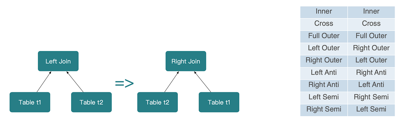
Rule 1: Join Commutativity

A join between two relations can be reordered by swapping its inputs:A JOIN B → B JOIN A

During this transformation, the join type must be adjusted accordingly. For example, a LEFT OUTER JOIN becomes a RIGHT OUTER JOIN after swapping the join operands.

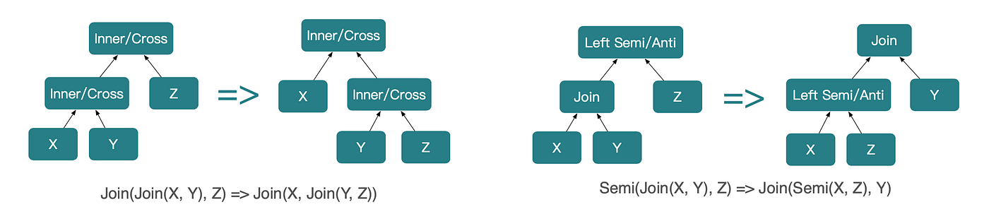
Rule 2: Join Associativity

Join associativity allows the join order among three relations to be rearranged:(A JOIN B) JOIN C → A JOIN (B JOIN C)

In StarRocks, associativity is handled differently depending on the join type. Specifically, StarRocks distinguishes between:

• Associativity for Inner / Cross Joins
• Associativity for Semi Joins
  
  

3.2 Greedy

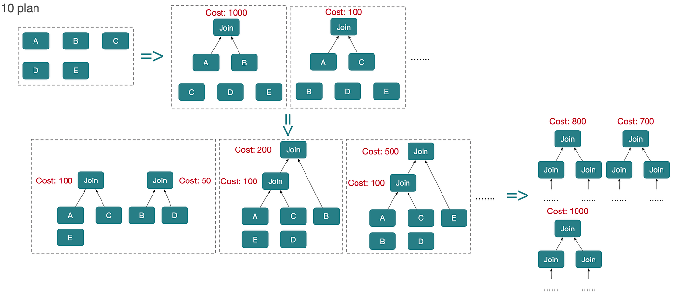
For its greedy join reordering strategy, StarRocks primarily draws inspiration from multi-sequence greedy algorithms, with a small but important enhancement: at each iteration level, instead of keeping only a single best result, StarRocks retains the top 10 candidate plans (which may not be globally optimal). These candidates are then carried forward into the next iteration, ultimately producing 10 greedy-optimized plans.

Due to the inherent limitations of greedy algorithms, this approach does not guarantee a globally optimal plan. However, by preserving multiple high-quality candidates at each step, it significantly increases the likelihood of finding a near-optimal or optimal solution.

Press enter or click to view image in full size

3.3 Cost Model

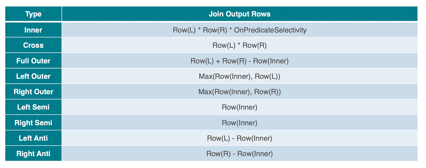
StarRocks uses these join reordering algorithms to generate N candidate plans. It then evaluates them with a cost model that estimates the cost of each join. The overall cost is computed as: Join Cost = CPU × (Row(L) + Row(R)) + Memory × Row(R)

Here, Row(L) and Row(R) are the estimated output row counts of the join’s left and right children, respectively. This formula primarily accounts for the CPU cost of processing both inputs, as well as the memory cost of building the hash table on the right side of a hash join. The figure below shows how StarRocks estimates join output row counts in more detail.

Because different join reordering algorithms explore search spaces of varying sizes and have different time complexities, StarRocks benchmarks their execution time and complexity characteristics, as shown below.

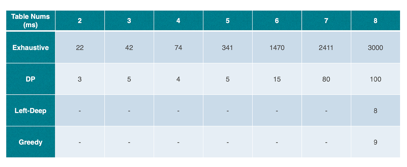
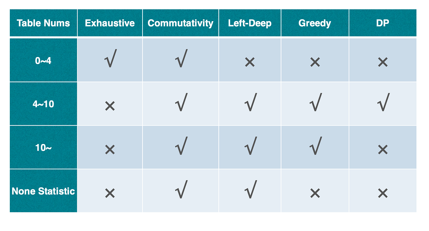
Based on the observed execution costs, StarRocks applies practical limits to how different join reordering algorithms are used:

• For joins involving up to 4 tables, StarRocks uses the exhaustive algorithm.
• For joins with 4–10 tables, StarRocks generates:
• 1 plan using the left-deep strategy,
• 10 plans using the greedy algorithm,
• 1 plan using dynamic programming.

On top of these, StarRocks further explores additional plans using join commutativity.

• For joins with more than 10 tables, StarRocks relies only on the greedy and left-deep strategies, producing a total of 11 candidate plans as the basis for reordering.
• When statistics are unavailable, cost-based greedy and dynamic programming approaches become unreliable. In this case, StarRocks falls back to using a single left-deep plan as the basis for join reordering.

Distributed Join Planning

After covering the logical optimizations involved in join queries, we now turn to join execution in a distributed environment, focusing on how StarRocks optimizes distributed join planning as a distributed database.

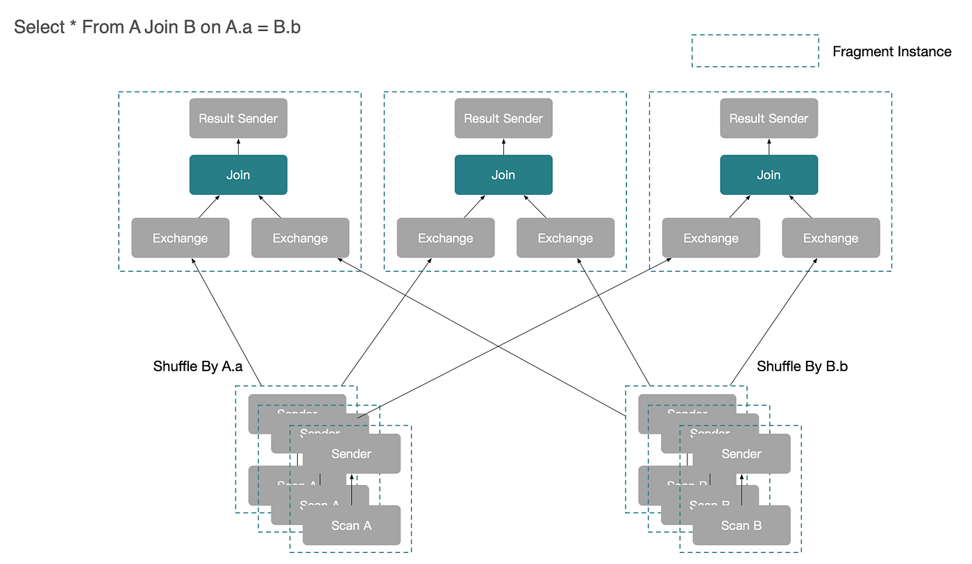
4.1 MPP Parallel Execution

StarRocks is built on an MPP (Massively Parallel Processing) execution framework. The overall architecture is illustrated below. Using a simple join query as an example, the execution of A JOIN B in StarRocks typically proceeds as follows:

• Data from tables A and B is read in parallel from different nodes, based on their respective data distributions.
• According to the join predicate, data from A and B is reshuffled so that matching rows are sent to the same set of nodes.
• The join is executed locally on each node, and the partial results are produced.

As shown, query execution usually involves multiple sets of machines: the nodes reading table A, the nodes reading table B, and the nodes performing the join are not necessarily the same. As a result, execution inevitably involves network transfers and data exchanges.

These network operations introduce significant overhead. Therefore, a key goal in optimizing distributed join execution in StarRocks is to minimize network cost, while more intelligently partitioning and distributing the query plan to fully leverage the benefits of parallel execution.

 

4.2 Distributed Join Optimization

We begin by introducing the distributed execution plans that StarRocks can generate. Using a simple join query as an example:

Select * From A Join B on A.a = B.b

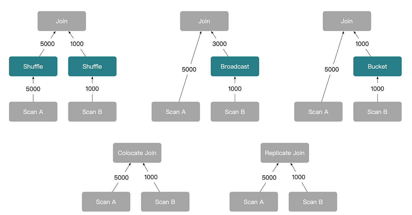
In practice, StarRocks can generate five basic types of distributed join plans:

• Shuffle Join Data from both tables A and B is shuffled based on the join key so that matching rows are sent to the same set of nodes, where the join is then executed.
• Broadcast Join The entire table B is broadcast to all nodes that hold table A, and the join is performed locally on those nodes. Compared to a shuffle join, this avoids shuffling table A, but requires broadcasting all of table B. This strategy is suitable when B is a small table.
• Bucket Shuffle Join An optimization over broadcast join. Instead of broadcasting table B to all nodes, B is shuffled according to A’s data distribution and sent only to the corresponding nodes that hold matching buckets of A. Globally, the shuffled data from B exists only once, significantly reducing network traffic compared to broadcast join. This strategy has an important constraint: the join key must be consistent with A’s distribution key.
• Colocate Join When tables A and B are created within the same colocate group, their data distributions are guaranteed to be identical. If the join key matches the distribution key, StarRocks can execute the join directly on the local nodes holding A and B, without any data shuffle.
• Replicate Join An experimental feature in StarRocks. If every node holding table A also contains a full copy of table B, the join can be executed locally. This approach has very strict requirements — essentially requiring the replication factor of table B to match the total number of nodes in the cluster — making it impractical in most real-world scenarios.

 

4.3 Exploring Distributed Join Plans

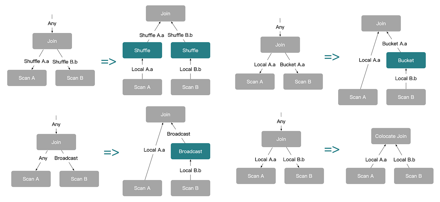
StarRocks derives distributed join plans through distribution property inference. Using a shuffle join as an example:SELECT * FROM A JOIN B ON A.a = B.b, the join operator propagates shuffle requirements top-down to tables A and B. If a scan node cannot satisfy the required distribution, StarRocks inserts an Enforce operator to introduce a shuffle. In the final execution plan, this shuffle is translated into an Exchange node responsible for network data transfer.

Other distributed join strategies are derived in the same way: the join operator requests different distribution properties from its input operators, and the optimizer generates the corresponding distributed execution plans accordingly.

 

 

4.4 Complex Distributed Joins

In real-world workloads, user queries are far more complex than a simple A JOIN B. They often involve three or more tables. For such queries, StarRocks generates a richer set of distributed execution plans, all derived from the same fundamental join strategies described earlier.

For example:

Select * From A Join B on A.a = B.b Join C on A.a = C.c

Using combinations of Shuffle Join and Broadcast Join, StarRocks can derive multiple distributed plans, as illustrated below.

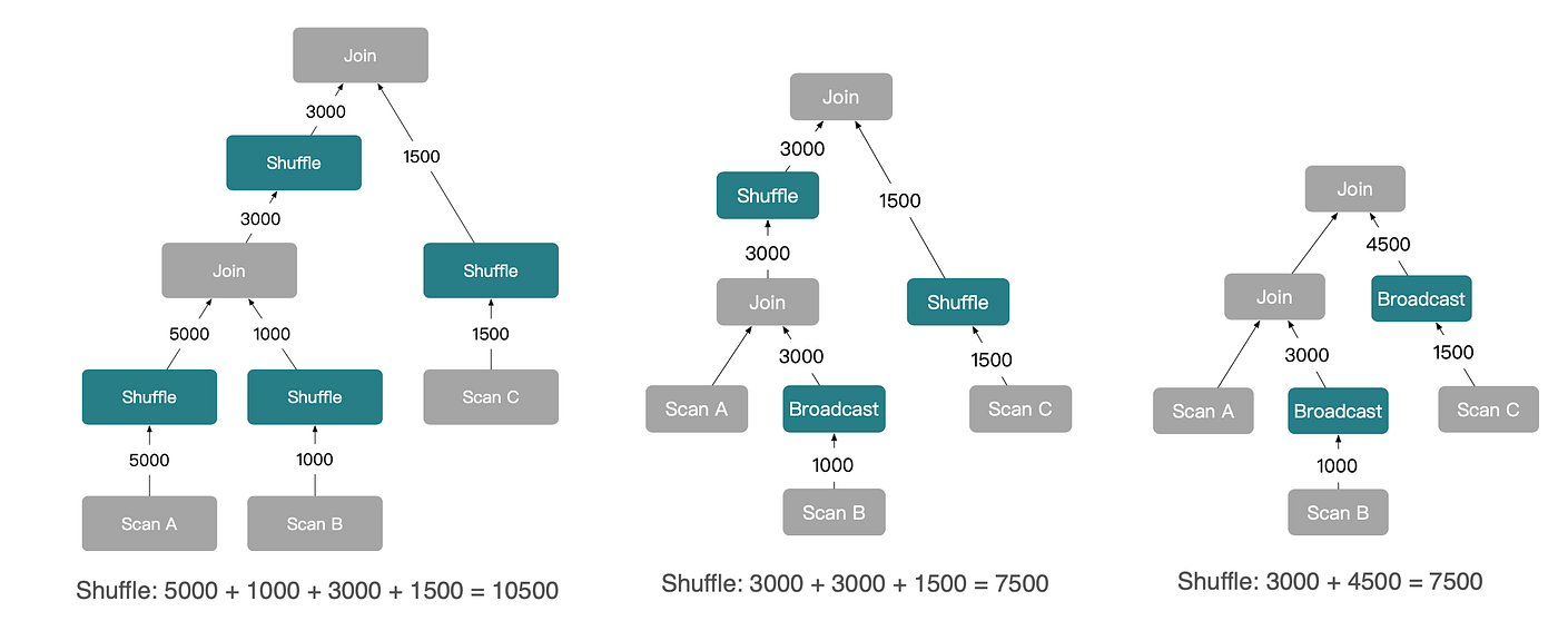
If Colocate Join and Bucket Shuffle Join are also considered, even more execution plans become possible:

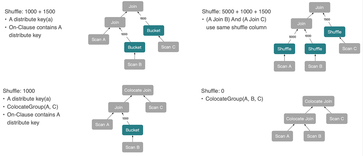
Despite their increased complexity, the underlying derivation logic remains the same. Distribution properties are propagated downward through the plan tree, allowing the optimizer to infer different combinations of distributed join strategies.

 

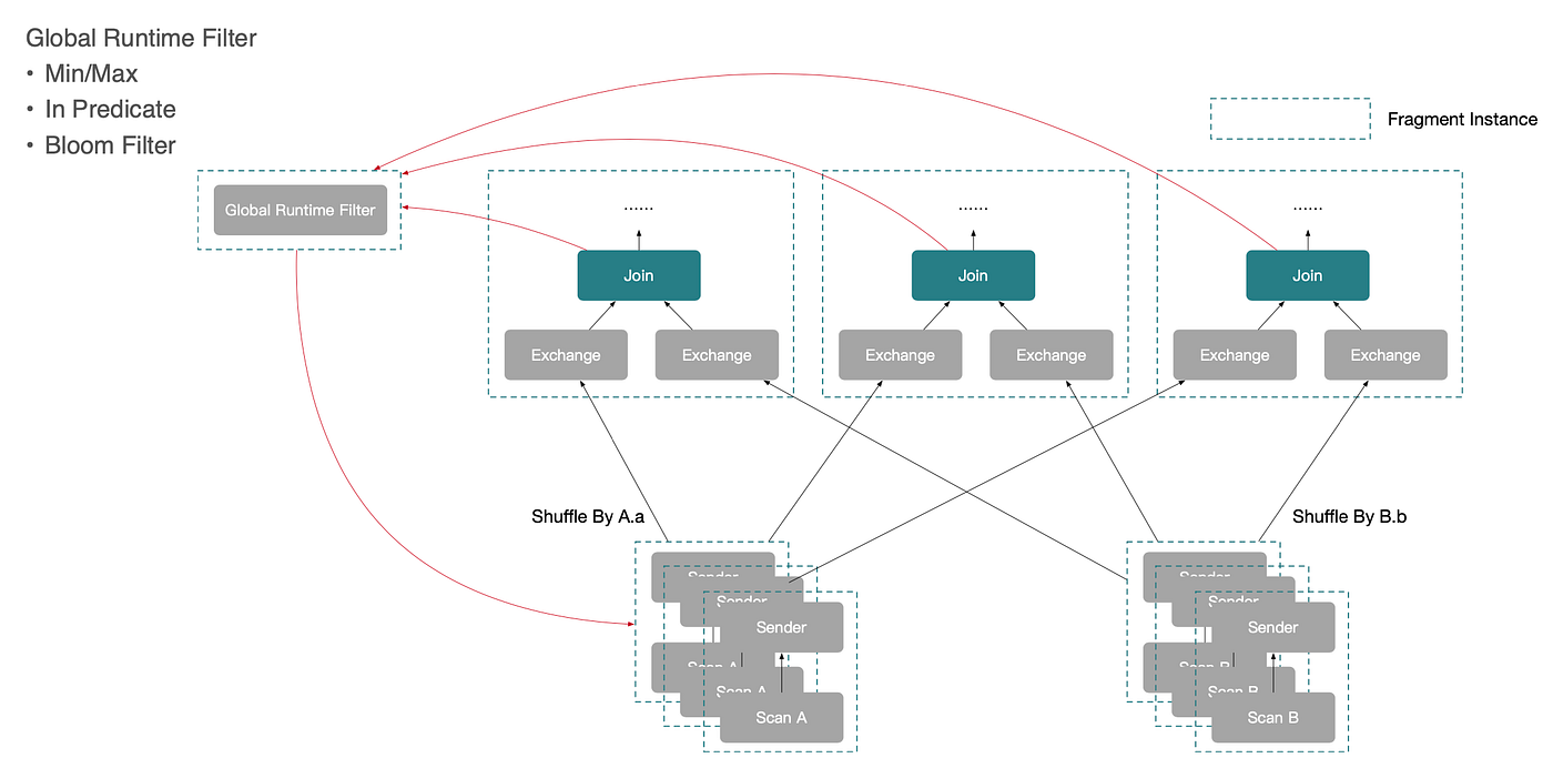
4.5 Global Runtime Filters

Beyond exploring distributed execution plans, StarRocks further optimizes join performance by leveraging the execution characteristics of join operators to build Global Runtime Filters.

The execution flow of a Hash Join in StarRocks is as follows:

1. Retrieve the complete data set from the right table.
2. Build a hash table from the right table.
3. Fetch data from the left table.
4. Probe the hash table to evaluate join conditions.
5. Produce the join results.

Global Runtime Filters are applied between Step 2 and Step 3. After constructing the hash table on the right side, StarRocks derives runtime filter predicates from the observed data and pushes these filters down to the scan nodes of the left table before left-side data is read. This allows the left table to filter out irrelevant rows early, significantly reducing join input size.

At present, Global Runtime Filters in StarRocks support the following filtering techniques: Min/Max filters, IN predicates, and Bloom filters. The diagram below illustrates how these filters work in practice.

Summary

This article has explored StarRocks’ practical experience and ongoing work in join query optimization. All of the techniques discussed are closely aligned with the core optimization principles outlined throughout the article. When optimizing SQL queries in practice, users can also apply the following guidelines together with the features provided by StarRocks to achieve better performance:

• Join operators vary significantly in performance. Prefer high-performance join types whenever possible and avoid expensive ones. Based on typical join output sizes, the rough performance ranking is: Semi Join / Anti Join > Inner Join > Outer Join > Full Outer Join > Cross Join.
• For hash joins, building the hash table on a smaller input is far more efficient than building it on a large table.
• In multi-table joins, execute highly selective joins first to substantially reduce the cost of subsequent joins.
• Minimize the amount of data participating in joins through early filtering and pruning.
• Reduce network overhead in distributed joins as much as possible to fully benefit from parallel execution.

 

Case Studies

Demandbase

By leveraging StarRocks’ On-the-Fly JOIN capabilities, Demandbase successfully replaced its existing ClickHouse clusters, optimizing performance while significantly reducing costs across multiple areas.

Read the case study: Demandbase Ditches Denormalization By Switching off ClickHouse

Naver

NAVER modernized its data infrastructure with StarRocks by enabling scalable, real-time analytics over multi-table joins without denormalization. The case study highlights the critical role of efficient, on-the-fly join execution in supporting production-scale analytical workloads.

Read the case study: How JOIN Changed How We Approach Data Infra At NAVER

Shopee

Data Go is a no-code query platform where Shopee business users build queries from multiple tables. Presto struggled with complex join performance and high resource usage. When Shopee switched to StarRocks for multi-table joins, they observed 3×–10× performance improvements and a ~60% reduction in CPU usage compared with Presto on external Hive data.

Read the case study: How Shopee 3xed Their Query Performance With StarRocks